facet_geo

Arrange a sequence of geographical panels into a grid that preserves some geographical orientation

Usage

facet_geo(facets, ..., grid = "us_state_grid1", label = NULL, move_axes = TRUE)

Arguments

facets

passed to facet_wrap

grid

character vector of the grid layout to use (currently only “us_state_grid1” and “us_state_grid2” are available)

label

an optional string denoting the name of a column in grid to use for facet labels. If NULL, the variable that best matches that in the data specified with facets will be used for the facet labels.

move_axes

should axis labels and ticks be moved to the closest panel along the margins?

…

additional parameters passed to facet_wrap

Examples

## Not run: 
# library(ggplot2)
# 
# # barchart of state rankings in various categories
# ggplot(state_ranks, aes(variable, rank, fill = variable)) +
#   geom_col() +
#   coord_flip() +
#   facet_geo(~ state) +
#   theme_bw()
# 
# # use an alternative US state grid and place
# ggplot(state_ranks, aes(variable, rank, fill = variable)) +
#   geom_col() +
#   coord_flip() +
#   facet_geo(~ state, grid = "us_state_grid2") +
#   theme(panel.spacing = unit(0.1, "lines"))
# 
# # custom grid (move Wisconsin above Michigan)
# my_grid <- us_state_grid1
# my_grid$col[my_grid$code == "WI"] <- 7
# 
# ggplot(state_ranks, aes(variable, rank, fill = variable)) +
#   geom_col() +
#   coord_flip() +
#   facet_geo(~ state, grid = my_grid)
# 
# # plot unemployment rate time series for each state
# ggplot(state_unemp, aes(year, rate)) +
#   geom_line() +
#   facet_geo(~ state) +
#   scale_x_continuous(labels = function(x) paste0("'", substr(x, 3, 4))) +
#   ylab("Unemployment Rate (%)") +
#   theme_bw()
# 
# # plot the 2016 unemployment rate
# ggplot(subset(state_unemp, year == 2016), aes(factor(year), rate)) +
#   geom_col(fill = "steelblue") +
#   facet_geo(~ state) +
#   theme(
#     axis.title.x = element_blank(),
#     axis.text.x = element_blank(),
#     axis.ticks.x = element_blank()) +
#   ylab("Unemployment Rate (%)") +
#   xlab("Year")
# 
# # plot European Union GDP
# ggplot(eu_gdp, aes(year, gdp_pc)) +
#   geom_line(color = "steelblue") +
#   geom_hline(yintercept = 100, linetype = 2) +
#   facet_geo(~ name, grid = "eu_grid1") +
#   scale_x_continuous(labels = function(x) paste0("'", substr(x, 3, 4))) +
#   ylab("GDP Per Capita") +
#   theme_bw()
# 
# # use a free x-axis to look at just change
# ggplot(eu_gdp, aes(year, gdp_pc)) +
#   geom_line(color = "steelblue") +
#   facet_geo(~ name, grid = "eu_grid1", scales = "free_y") +
#   scale_x_continuous(labels = function(x) paste0("'", substr(x, 3, 4))) +
#   ylab("GDP Per Capita in Relation to EU Index (100)") +
#   theme_bw()
# # would be nice if ggplot2 had a "sliced" option...
# # (for example, there's not much going on with Denmark but it looks like there is)
# 
# # plot European Union annual # of resettled persons
# ggplot(eu_imm, aes(year, persons)) +
#   geom_line() +
#   facet_geo(~ name, grid = "eu_grid1") +
#   scale_x_continuous(labels = function(x) paste0("'", substr(x, 3, 4))) +
#   scale_y_sqrt(minor_breaks = NULL) +
#   ylab("# Resettled Persons") +
#   theme_bw()
# 
# # plot just for 2016
# ggplot(subset(eu_imm, year == 2016), aes(factor(year), persons)) +
#   geom_col(fill = "steelblue") +
#   geom_text(aes(factor(year), 3000, label = persons), color = "gray") +
#   facet_geo(~ name, grid = "eu_grid1") +
#   theme(
#     axis.title.x = element_blank(),
#     axis.text.x = element_blank(),
#     axis.ticks.x = element_blank()) +
#   ylab("# Resettled Persons in 2016") +
#   xlab("Year") +
#   theme_bw()
# 
# # plot Australian population
# ggplot(aus_pop, aes(age_group, pop / 1e6, fill = age_group)) +
#   geom_col() +
#   facet_geo(~ code, grid = "aus_grid1") +
#   coord_flip() +
#   labs(
#     title = "Australian Population Breakdown",
#     caption = "Data Source: ABS Labour Force Survey, 12 month average",
#     y = "Population [Millions]") +
#   theme_bw()
# 
# # South Africa population density by province
# ggplot(sa_pop_dens, aes(factor(year), density, fill = factor(year))) +
#   geom_col() +
#   facet_geo(~ province, grid = "sa_prov_grid1") +
#   labs(title = "South Africa population density by province",
#     caption = "Data Source: Statistics SA Census",
#     y = "Population density per square km") +
#   theme_bw()
# 
# # use the Afrikaans name stored in the grid, "name_af", as facet labels
# ggplot(sa_pop_dens, aes(factor(year), density, fill = factor(year))) +
#   geom_col() +
#   facet_geo(~ code, grid = "sa_prov_grid1", label = "name_af") +
#   labs(title = "South Africa population density by province",
#     caption = "Data Source: Statistics SA Census",
#     y = "Population density per square km") +
#   theme_bw()
# 
# # affordable housing starts by year for boroughs in London
# ggplot(london_afford, aes(x = year, y = starts, fill = year)) +
#   geom_col(position = position_dodge()) +
#   facet_geo(~ code, grid = "london_boroughs_grid", label = "name") +
#   labs(title = "Affordable Housing Starts in London",
#     subtitle = "Each Borough, 2015-16 to 2016-17",
#     caption = "Source: London Datastore", x = "", y = "")
# 
# # dental health in Scotland
# ggplot(nhs_scot_dental, aes(x = year, y = percent)) +
#   geom_line() +
#   facet_geo(~ name, grid = "nhs_scot_grid") +
#   scale_x_continuous(breaks = c(2004, 2007, 2010, 2013)) +
#   scale_y_continuous(breaks = c(40, 60, 80)) +
#   labs(title = "Child Dental Health in Scotland",
#     subtitle = "Percentage of P1 children in Scotland with no obvious decay experience.",
#     caption = "Source: statistics.gov.scot", x = "", y = "")
# 
# # India population breakdown
# ggplot(subset(india_pop, type == "state"),
#   aes(pop_type, value / 1e6, fill = pop_type)) +
#   geom_col() +
#   facet_geo(~ name, grid = "india_grid1", label = "code") +
#   labs(title = "Indian Population Breakdown",
#        caption = "Data Source: Wikipedia",
#        x = "",
#        y = "Population [Millions]") +
#   theme_bw() +
#   theme(axis.text.x = element_text(angle = 40, hjust = 1))
# 
# ggplot(subset(india_pop, type == "state"),
#   aes(pop_type, value / 1e6, fill = pop_type)) +
#   geom_col() +
#   facet_geo(~ name, grid = "india_grid2", label = "name") +
#   labs(title = "Indian Population Breakdown",
#        caption = "Data Source: Wikipedia",
#        x = "",
#        y = "Population [Millions]") +
#   theme_bw() +
#   theme(axis.text.x = element_text(angle = 40, hjust = 1),
#     strip.text.x = element_text(size = 6))
# 
# # A few ways to look at the 2016 election results
# ggplot(election, aes("", pct, fill = candidate)) +
#   geom_col(alpha = 0.8, width = 1) +
#   scale_fill_manual(values = c("#4e79a7", "#e15759", "#59a14f")) +
#   facet_geo(~ state, grid = "us_state_grid2") +
#   scale_y_continuous(expand = c(0, 0)) +
#   labs(title = "2016 Election Results",
#     caption = "Data Source: http://bit.ly/2016votecount",
#     x = NULL,
#     y = "Percentage of Voters") +
#   theme(axis.title.x = element_blank(),
#     axis.text.x = element_blank(),
#     axis.ticks.x = element_blank(),
#     strip.text.x = element_text(size = 6))
# 
# ggplot(election, aes(candidate, pct, fill = candidate)) +
#   geom_col() +
#   scale_fill_manual(values = c("#4e79a7", "#e15759", "#59a14f")) +
#   facet_geo(~ state, grid = "us_state_grid2") +
#   theme_bw() +
#   coord_flip() +
#   labs(title = "2016 Election Results",
#     caption = "Data Source: http://bit.ly/2016votecount",
#     x = NULL,
#     y = "Percentage of Voters") +
#   theme(strip.text.x = element_text(size = 6))
# 
# ggplot(election, aes(candidate, votes / 1000000, fill = candidate)) +
#   geom_col() +
#   scale_fill_manual(values = c("#4e79a7", "#e15759", "#59a14f")) +
#   facet_geo(~ state, grid = "us_state_grid2") +
#   coord_flip() +
#   labs(title = "2016 Election Results",
#     caption = "Data Source: http://bit.ly/2016votecount",
#     x = NULL,
#     y = "Votes (millions)") +
#   theme(strip.text.x = element_text(size = 6))
# ## End(Not run)

get_grid_names

Get a list of valid grid names

Usage

get_grid_names()

grid_design

Interactively design a grid

Usage

grid_design(data = NULL, img = NULL, label = "code", auto_img = TRUE)

Arguments

data

A data frame containing a grid to start from or NULL if starting from scratch.

img

An optional URL pointing to a reference image containing a geographic map of the entities in the grid.

label

An optional column name to use as the label for plotting the original geography, if attached to data.

auto_img

If the original geography is attached to data, should a plot of that be created and uploaded to the viewer?

Examples

# edit aus_grid1
grid_design(data = aus_grid1, img = "http://www.john.chapman.name/Austral4.gif")
# start with a clean slate
grid_design()
# arrange the alphabet
grid_design(data.frame(code = letters))

grid_preview

Plot a preview of a grid

Usage

grid_preview(x, label = NULL, label_raw = NULL)

Arguments

x

a data frame containing a grid

label

the column name in x that should be used for text labels in the grid plot

label_raw

the column name in the optional SpatialPolygonsDataFrame attached to x that should be used for text labels in the raw geography plot

Examples

grid_preview(us_state_grid2)

## Note: You provided a user-specified grid. If this is a generally-useful
##   grid, please consider submitting it to become a part of the geofacet
##   package. You can do this easily by calling:
##   grid_submit(__grid_df_name__)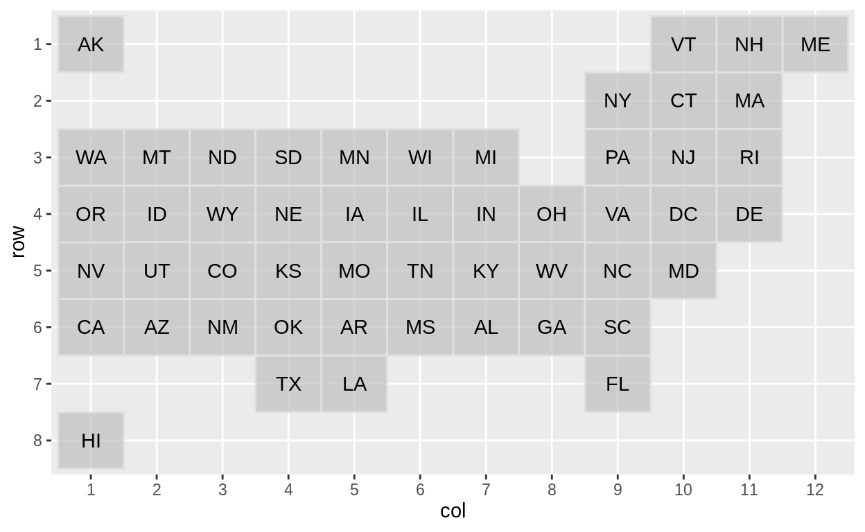

grid_preview(eu_grid1, label = "name")

## Note: You provided a user-specified grid. If this is a generally-useful
##   grid, please consider submitting it to become a part of the geofacet
##   package. You can do this easily by calling:
##   grid_submit(__grid_df_name__)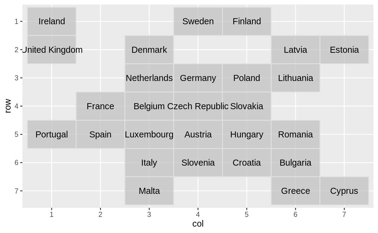

grid_submit

Submit a grid to be included in the package

Usage

grid_submit(x, name = NULL, desc = NULL)

Arguments

x

a data frame containing a grid

name

proposed name of the grid (if not supplied, will be asked for interactively)

desc

a description of the grid (if not supplied, will be asked for interactively)

Details

This opens up a github issue for this package in the web browser with pre-populated content for adding a grid to the package.

Examples

## Not run: 
# my_grid <- us_state_grid1
# my_grid$col[my_grid$label == "WI"] <- 7
# grid_submit(my_grid, name = "us_grid_tweak_wi",
#   desc = "Modified us_state_grid1 to move WI over")
# ## End(Not run)

grids

Geo Grids

There are now 64 grids available in this package and more online. To view a full list of available grids, see here. To create and submit your own grid, see here. To see several examples of grids being used to visualize data, see facet_geo.

• us_state_grid1: Grid layout for US states (including DC) Image reference here.

• us_state_grid2: Grid layout for US states (including DC) Image reference here.

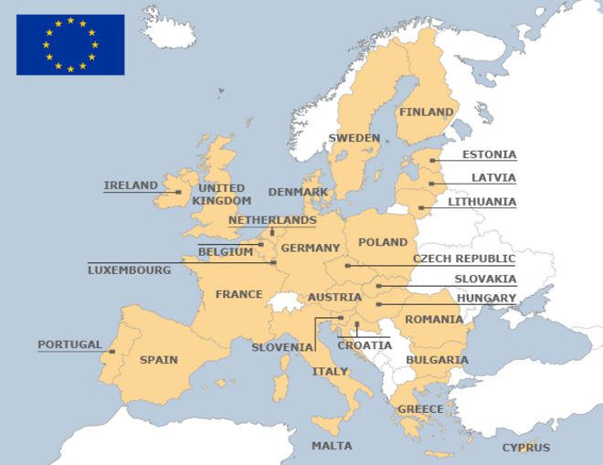
• eu_grid1: Grid layout for the 28 EU Countries Image reference here.

• aus_grid1: Grid layout for the Australian States and Territories. Image reference here. Thanks to jonocarroll.

• sa_prov_grid1: Grid layout for the provinces of South Africa Image reference here. Thanks to jonmcalder.

• london_boroughs_grid: Grid layout for the boroughs of London. Note that the column code_ons contains the codes used by UK Office for National Statistics. Image reference here. Thanks to eldenvo.

• nhs_scot_grid: Grid layout for a grid of NHS Scotland Health Boards. Note that the column code contains the codes used by UK Office for National Statistics. Image reference here. Thanks to jsphdms.

• india_grid1: Grid layout for India states (not including union territories). Image reference here. Thanks to meysubb.

• india_grid2: Grid layout for India states (not including union territories). Image reference here.

• argentina_grid1: Grid for the 23 provinces of Argentina. It includes the Malvinas/Falkland Islands and the Antarctic Territories (these are disputed, but they are included since many researchers might use data from these locations). Image reference here. Thanks to eliocamp.

• br_states_grid1: Grid for the 27 states of Brazil. Image reference here. Thanks to italocegatta.

• sea_grid1: Grid for South East Asian countries. Image reference here. Thanks to jasonjb82.

• mys_grid1: Grid for Malaysian states and territories. Image reference here. Thanks to jasonjb82.

• fr_regions_grid1: Land and overseas regions of France. Codes are INSEE codes. Image reference here. Thanks to mtmx.

• de_states_grid1: Grid for the German states (‘Länder’) Image reference here. Thanks to DominikVogel.

• us_or_counties_grid1: Grid for Oregon counties. Image reference here. Thanks to aosmith16.

• us_wa_counties_grid1: Grid for Washington counties. Image reference here.

• us_in_counties_grid1: Grid for Indiana counties. Image reference here. Thanks to nateapathy.

• us_in_central_counties_grid1: Grid for central Indiana counties. Image reference here. Thanks to nateapathy.

• se_counties_grid1: Grid for counties of Sweden. Image reference here. Thanks to duleise.

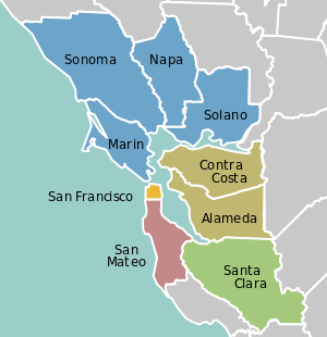
• sf_bay_area_counties_grid1: Grid of the 9 San Francisco Bay Area counties. Image reference here. Thanks to Eunoia.

• ua_region_grid1: Grid of administrative divisions of Ukraine (24 oblasts, one autonomous region, and two cities). Image reference here. Thanks to woldemarg.

• mx_state_grid1: Grid layout for the states of Mexico. Image reference here. Thanks to ikashnitsky.

• mx_state_grid2: Grid layout for the states of Mexico. Image reference here. Thanks to diegovalle.

• scotland_local_authority_grid1: Grid layout for the local authorities of Scotland. Image reference here. Thanks to davidhen.

• us_state_grid3: Grid layout for US states (excluding DC) Image reference here. Thanks to ejr248.

• italy_grid1: Grid layout for regions of Italy (in collaboration with Stella Cangelosi and Luciana Dalla Valle). Image reference here. Thanks to JulianStander.

• italy_grid2: Grid layout for regions of Italy (in collaboration with Stella Cangelosi and Luciana Dalla Valle). Image reference here. Thanks to JulianStander.

• be_province_grid1: Grid layout for provinces of Belgium plus Brussels, including names in three languages (French, Dutch, English) and Belgium internal codes (NIS). Image reference here. Thanks to ericlecoutre.

• us_state_grid4: Grid layout for US states (including DC). Image reference here. Thanks to kanishkamisra.

• jp_prefs_grid1: Grid layout for the prefectures of Japan. Image reference here. Thanks to uribo.

• ng_state_grid1: Grid layout for the 37 Federal States of Nigeria. Image reference here. Thanks to ghosthedirewolf.

• bd_upazila_grid1: Grid layout for Bangladesh 64 Upazilas. Image reference here. Thanks to ghosthedirewolf.

• spain_prov_grid1: Grid layout for Provinces of Spain. Image reference here. Thanks to kintero.

• ch_cantons_grid1: Grid layout for Cantons of Switzerland. Image reference here. Thanks to tinu-schneider.

• ch_cantons_grid2: Grid layout for Cantons of Switzerland. Image reference here. Thanks to rastrau.

• china_prov_grid1: Grid layout for Provinces of China. Image reference here. Thanks to weiyunna.

• world_86countries_grid: Grid layout for 86 countries in the world. Image reference here. Thanks to akangsha.

• se_counties_grid2: Grid for counties of Sweden. Image reference here. Thanks to richardohrvall.

• uk_regions1: Grid for regions of the UK (aka EU standard NUTS 1 areas). Image reference here. Thanks to paulb20.

• us_state_contiguous_grid1: Grid layout for the contiguous US states (including DC). Image reference here. Thanks to andrewsr.

• sk_province_grid1: Grid layout for South Korean sis and dos (metropolitan/special/autonomous cities and provinces). Image reference here. Thanks to heon131.

• ch_aargau_districts_grid1: Grid layout for Districts of the Canton of Aargau, Switzerland. Image reference here. Thanks to zumbov2.

• jo_gov_grid1: Grid layout for Governorates of Jordan. Image reference here. Thanks to ghosthedirewolf.

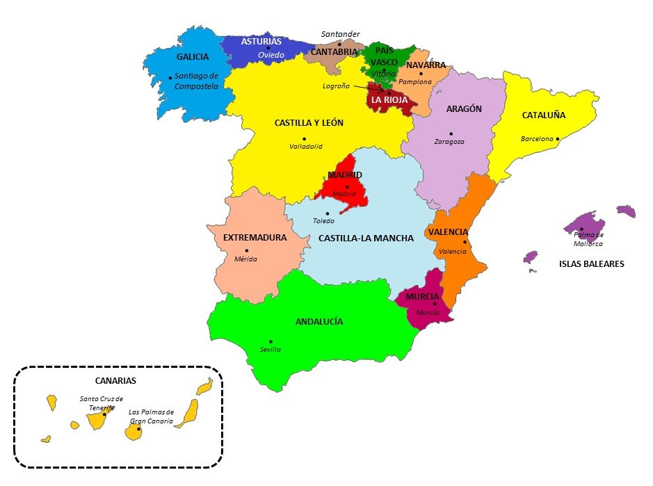
• spain_ccaa_grid1: Grid layout for Spanish ‘Comunidades Autónomas’. Image reference here. Thanks to JoseAntonioOrtega.

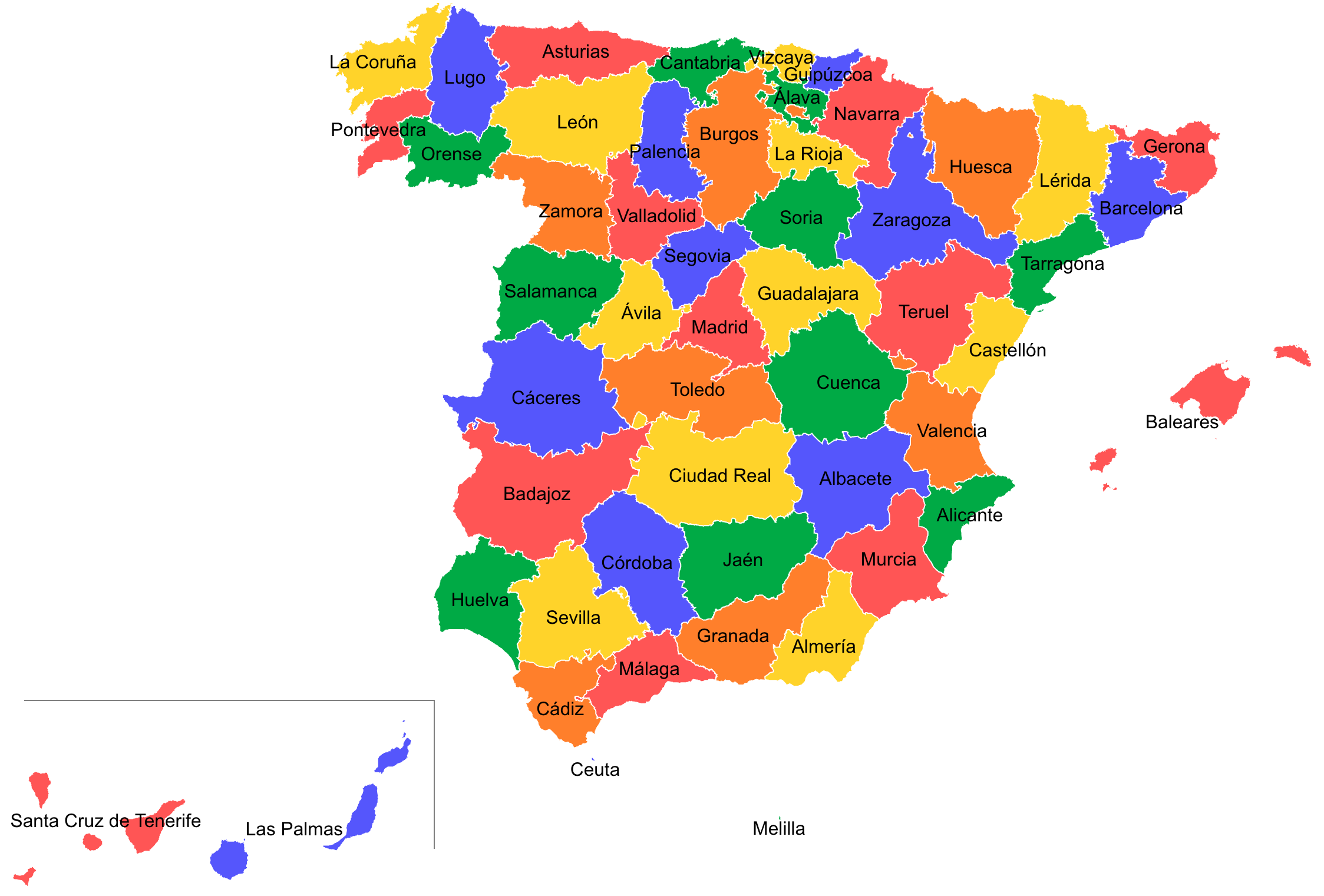
• spain_prov_grid2: Grid layout for Provinces of Spain. Image reference here. Thanks to JoseAntonioOrtega.

• world_countries_grid1: Grid layout for countries of the world, with a few exclusions. See . Image reference here. Thanks to JoseAntonioOrtega.

• br_states_grid2: Grid for the 27 states of Brazil. Image reference here. Thanks to hafen.

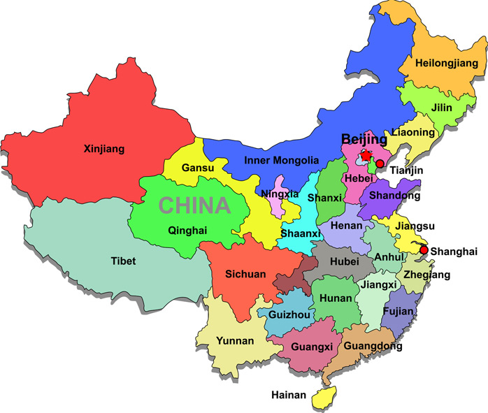
• china_city_grid1: Grid layout of cities in China. Image reference here. Thanks to CharleneDeng1.

• kr_seoul_district_grid1: Grid layout of Seoul’s 25 districts. Image reference here. Thanks to yonghah.

• nz_regions_grid1: Grid layout for regions of New Zealand. Image reference here. Thanks to pierreroudier.

• sl_regions_grid1: Grid layout of Slovenian regions. Image reference here. Thanks to SR1986.

• us_census_div_grid1: Grid layout of US Census divisions. Image reference here. Thanks to mkiang.

• ar_tucuman_province_grid1: Grid layout for Argentina Tucumán Province political divisions (departments) Image reference here. Thanks to TuQmano.

• us_nh_counties_grid1: Grid layout for the 10 counties in New Hampshire. Image reference here. Thanks to soungl.

• china_prov_grid2: Grid layout for Provinces of China. Image reference here. Thanks to jw2531.

• pl_voivodeships_grid1: Grid layout for Polish voivodeships (provinces) Image reference here. Thanks to erzk.

• us_ia_counties_grid1: Grid layout for counties in Iowa Image reference here. Thanks to jrennyb.

• us_id_counties_grid1: Grid layout for counties in Idaho Image reference here. Thanks to hathawayj.

• ar_cordoba_dep_grid1: Grid layout for departments of Cordoba province in Argentina. Image reference here. Thanks to TuQmano.

• us_fl_counties_grid1: Grid for Florida counties. Image reference here. Thanks to ejr248.

• ar_buenosaires_communes_grid1: Grid for communes of Buenos Aires, Argentina. Image reference here. Thanks to TuQmano.

• nz_regions_grid2: Grid layout for regions of New Zealand. Image reference here. Thanks to pierreroudier.

• oecd_grid1: Grid layout for OECD member countries. Image reference here. Thanks to arcruz0.

Usage

us_state_grid1
us_state_grid2
eu_grid1
aus_grid1
sa_prov_grid1
london_boroughs_grid
nhs_scot_grid
india_grid1
india_grid2
argentina_grid1
br_states_grid1
sea_grid1
mys_grid1
fr_regions_grid1
de_states_grid1
us_or_counties_grid1
us_wa_counties_grid1
us_in_counties_grid1
us_in_central_counties_grid1
se_counties_grid1
sf_bay_area_counties_grid1
ua_region_grid1
mx_state_grid1
mx_state_grid2
scotland_local_authority_grid1
us_state_grid3
italy_grid1
italy_grid2
be_province_grid1
us_state_grid4
jp_prefs_grid1
ng_state_grid1
bd_upazila_grid1
spain_prov_grid1
ch_cantons_grid1
ch_cantons_grid2
china_prov_grid1
world_86countries_grid
se_counties_grid2
uk_regions1
us_state_contiguous_grid1
sk_province_grid1
ch_aargau_districts_grid1
jo_gov_grid1
spain_ccaa_grid1
spain_prov_grid2
world_countries_grid1
br_states_grid2
china_city_grid1
kr_seoul_district_grid1
nz_regions_grid1
sl_regions_grid1
us_census_div_grid1
ar_tucuman_province_grid1
us_nh_counties_grid1
china_prov_grid2
pl_voivodeships_grid1
us_ia_counties_grid1
us_id_counties_grid1
ar_cordoba_dep_grid1
us_fl_counties_grid1
ar_buenosaires_communes_grid1
nz_regions_grid2
oecd_grid1

aus_pop

aus_pop

March 2017 population data for Australian states and territories by age group. Source: http://lmip.gov.au/default.aspx?LMIP/Downloads/ABSLabourForceRegion.

Usage

aus_pop

election

election

2016 US presidential election results, obtained from http://bit.ly/2016votecount.

Usage

election

eu_gdp

eu_gdp

GDP per capita in PPS - Index (EU28 = 100). “Gross domestic product (GDP) is a measure for the economic activity. It is defined as the value of all goods and services produced less the value of any goods or services used in their creation. The volume index of GDP per capita in Purchasing Power Standards (PPS) is expressed in relation to the European Union (EU28) average set to equal 100. If the index of a country is higher than 100, this country’s level of GDP per head is higher than the EU average and vice versa. Basic figures are expressed in PPS, i.e. a common currency that eliminates the differences in price levels between countries allowing meaningful volume comparisons of GDP between countries. Please note that the index, calculated from PPS figures and expressed with respect to EU28 = 100, is intended for cross-country comparisons rather than for temporal comparisons.” Source: http://ec.europa.eu/eurostat/web/national-accounts/data/main-tables. Dataset ID: tec00114.

Usage

eu_gdp

eu_imm

eu_imm

Annual number of resettled persons for each EU country. “Resettled refugees means persons who have been granted an authorization to reside in a Member State within the framework of a national or Community resettlement scheme.”. Source: http://ec.europa.eu/eurostat/cache/metadata/en/migr_asydec_esms.htm. Dataset ID: tps00195.

Usage

eu_imm

india_pop

india_pop

2011 population data for India, broken down by urban and rural. Source: https://en.wikipedia.org/wiki/List_of_states_and_union_territories_of_India_by_population.

Usage

india_pop

london_afford

london_afford

Total affordable housing completions by financial year in each London borough since 2015/16. Source: https://data.london.gov.uk/dataset/dclg-affordable-housing-supply-borough

Usage

london_afford

nhs_scot_dental

nhs_scot_dental

Child dental health data in Scotland. Source: http://statistics.gov.scot/data/child-dental-health

Usage

nhs_scot_dental

sa_pop_dens

sa_pop_dens

Population density for each province in South Africa for 1996, 2001, and 2011. Source: https://en.wikipedia.org/wiki/List_of_South_African_provinces_by_population_density

Usage

sa_pop_dens

state_ranks

state_ranks

State rankings in the following categories with the variable upon which ranking is based in parentheses: education (adults over 25 with a bachelor’s degree in 2015), employment (March 2017 unemployment rate - Bureau of Labor Statistics), health (obesity rate from 2015 - Centers for Disease Control), insured (uninsured rate in 2015 - US Census), sleep (share of adults that report at least 7 hours of sleep each night from 2016 - Disease Control), wealth (poverty rate 2014/15 - US Census). In each category, the lower the ranking, the more favorable. This data is based on data presented here: https://www.axios.com/an-emoji-built-from-data-for-every-state-2408885674.html

Usage

state_ranks

state_unemp

state_unemp

Seasonally-adjusted December unemployment rate for each state (including DC) from 2000 to 2017. Obtained from bls.gov.

Usage

state_unemp